Tip: 0.3 represents the difference analysis between the 30 % samples with the highest MKI67 expression and the 30 % samples with the lowest MKI67 expression. If you want to use the median value analysis, you only need to change 0.3 to 0.5.
Background: In cancer pathway research, a broad screening strategy is typically employed during the initial analysis. Key pathway gene sets are usually documented in authoritative databases such as GO, KEGG, or Reactome. To validate the association between pathways and target genes, gene sets from these databases can be selected for Gene Set Enrichment Analysis (GSEA) across multiple independent datasets. GSEA evaluates the enrichment of gene sets within phenotype-related gene lists to determine their relevance to specific phenotypes or biological processes. If GSEA results from multiple datasets show consistent enrichment patterns, it suggests a significant association between the target gene and the pathway. This multi-dataset consistency analysis provides robust evidence for subsequent mechanistic studies, facilitating a systematic understanding of the role of target genes in cancer development and progression, and laying the groundwork for experimental validation and clinical applications.
The full version of disease abbreviations:
- Vitiligo: VL
- Psoriasis: PR
- Scleroderma: SD
- Dermatomyositis: DM
- Atopic Dermatitis: AD
- Systemic lupus erythematosus: SLE
You may cite:
- Literature: Lee E, Chuang HY, Kim JW, Ideker T, Lee D. Inferring pathway activity toward precise disease classification. PLoS Comput Biol. 2008;4(11):e1000217. doi: 10.1371/journal.pcbi.1000217. http://dx.doi.org/10.1371/journal.pcbi.1000217
Result interpretation
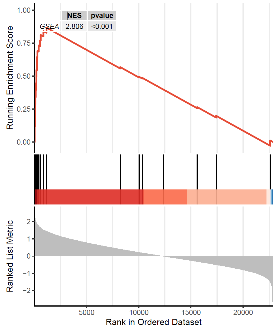
Figure legends: Enrichment of the gene set at the top, indicated by a positive ES/NES, suggests that the core molecules in the custom gene set are predominantly concentrated in the left-sided high-expression group. This implies significant enrichment of the target pathway in the high-expression group, indicating its activation in the high-expression group and suppression in the low-expression group.
Methods: Samples are first divided into high- and low-expression groups based on MKI67 expression levels, with the top 30% and bottom 30% of samples defined as high- and low-expression groups, respectively. To identify differentially expressed genes between the two groups, the limma package in R is used for differential expression analysis. During this process, the Delta value of the average Z-score for each gene is calculated between the high- and low-expression groups, reflecting the magnitude of gene expression changes. After differential expression analysis, all genes are ranked by their Delta values to prepare for subsequent Gene Set Enrichment Analysis (GSEA). The ranked gene list provides a clear representation of gene expression trends, facilitating the identification of significantly enriched gene sets. The GSEA function from the clusterProfiler package is then employed to perform gene set enrichment analysis based on custom gene sets. The Normalized Enrichment Score (NES) is calculated for each gene set, followed by significance testing and multiple hypothesis correction. These statistical tests help evaluate the enrichment levels of gene sets between the high- and low-expression groups, thereby identifying biological processes or metabolic pathways that exhibit significant differences between the two sample groups.
Results: The results demonstrate significant differences in the custom gene set between the high- and low-expression groups. These findings provide critical insights into the biological functions of MKI67 within the custom gene set and lay the foundation for further functional studies and potential clinical applications. Additionally, the results reveal key biological processes potentially regulated by MKI67, offering new research directions for future investigations.
R Code
Study
Statistics
More
GeneName = commandArgs(trailingOnly = TRUE)[1]
pctName = commandArgs(trailingOnly = TRUE)[2]
pct = as.numeric(pctName)
CustomName = as.vector(commandArgs(trailingOnly = TRUE)[2:(length(commandArgs(trailingOnly = TRUE))-1)])
DiseaseName = commandArgs(trailingOnly = TRUE)[length(commandArgs(trailingOnly = TRUE))]
options(warn = -1);startTime = Sys.time();startTime = as.character(startTime);startTime = gsub(" " ,"-",startTime);startTime = gsub(":" ,"-",startTime);dir.create(paste0(startTime));picDir = paste0(startTime);setwd(picDir)
OutputName = paste0(startTime,"_",GeneName,"_",pctName,"_",DiseaseName,"_gsea_custom_geneset")
library(fromto)
customized_geneset = customized(CustomName)
#GeneName = "MKI67";DiseaseName = "SLE"
if(DiseaseName == "VL"){
  load("Vitiligo.Rdata")
  levels_use = c("Vitiligo","Vitiligo-lesional","Vitiligo-nonlesional","Vitiligo-perilesional","Vitiligo-Generalized","Vitiligo-Segmental","Healthy")
}else if(DiseaseName == "PR"){
  load("SkinDB_Psoriasis.RData")
  expression_zscore = expression_renew_zscore
  rm(expression_renew_zscore)
  levels_use = c("Psoriasis","Healthy")
}else if(DiseaseName == "SD"){
  load("Scleroderma.Rdata")
  levels_use = c("Scleroderma","Sclerotic-Skin","Inflammatory-Border","Nonlesional-Skin","Responder","Non-responder","Baseline","Post-Gleevec","Pre-Gleevec","Nilotinib","Abatacept","Week3-4","Week7","Week24","Tadalafil","C82","Dasatinib","Belimumab","Scleroderma-Baseline","Scleroderma-Transplant","Scleroderma-Cyclophosphamide","Placebo","Healthy")
}else if(DiseaseName == "DM"){
  load("DM.Rdata")
  levels_use = c("JDM","DM","DM-active","Healthy")
}else if(DiseaseName == "AD"){
  load("AD.Rdata")
  levels_use = c("AD","AD-lesional","AD-lesional-acute","AD-lesional-chronic","AD-nonlesional","AD-betamethasone-treat","AD-pimecrolimus-treat","Dupilumab","ASN002-20mg","ASN002-40mg","ASN002-80mg","Crisaborole","Ustekinumab","Vehicle","Placebo","Treated","Untreated","Healthy")
}else if(DiseaseName == "SLE"){
  load("SLE.Rdata")
  levels_use = c("SLE","RBP+SLE","RBP-SLE","Lesional","Non-lesional","Nonlesional","AMG811","Placebo","Lupus-Nephritis","Healthy")
}

datasets = names(expression_zscore)
for (variable in datasets) {
  data = expression_zscore[[variable]]
  data = na.omit(data)
  if(GeneName %in% rownames(data)){
    if(DiseaseName == "VL"){
      data_subset = data[,which(strsplit_fromto(colnames(data),"_",2) %in% c("Vitiligo","Vitiligo-lesional","Vitiligo-nonlesional","Vitiligo-perilesional","Vitiligo-Generalized","Vitiligo-Segmental"))]
    }else if(DiseaseName == "PR"){
      data_subset = data[,which(strsplit_fromto(colnames(data),"_",2) == "Psoriasis")]
    }else if(DiseaseName == "SD"){
      data_subset = data[,which(strsplit_fromto(colnames(data),"_",2) %in% c("Scleroderma","Sclerotic-Skin","Inflammatory-Border","Nonlesional-Skin","Responder","Non-responder","Baseline","Post-Gleevec","Pre-Gleevec","Nilotinib","Abatacept","Week3-4","Week7","Week24","Tadalafil","C82","Dasatinib","Belimumab","Scleroderma-Baseline","Scleroderma-Transplant","Scleroderma-Cyclophosphamide","Placebo"))]
    }else if(DiseaseName == "DM"){
      data_subset = data[,which(strsplit_fromto(colnames(data),"_",2) %in% c("JDM","DM","DM-active"))]
    }else if(DiseaseName == "AD"){
      data_subset = data[,which(strsplit_fromto(colnames(data),"_",2) %in% c("AD","AD-lesional","AD-lesional-acute","AD-lesional-chronic","AD-nonlesional","AD-betamethasone-treat","AD-pimecrolimus-treat","Dupilumab","ASN002-20mg","ASN002-40mg","ASN002-80mg","Crisaborole","Ustekinumab","Vehicle","Placebo","Treated","Untreated"))]
    }else if(DiseaseName == "SLE"){
      data_subset = data[,which(strsplit_fromto(colnames(data),"_",2) %in% c("SLE","RBP+SLE","RBP-SLE","Lesional","Non-lesional","Nonlesional","AMG811","Placebo","Lupus-Nephritis"))]
    }

    if(ncol(data_subset) > 10 && length(intersect(CustomName,rownames(data_subset))) > 1){
      limma_gene_gsea_customized(data = data_subset,
                                 GeneName = GeneName,
                                 customized = customized_geneset,
                                 pct = pct,
                                 DatasetName = variable)
    }
  }
}


file.remove("Rplots.pdf");files = dir();zip(paste0(paste0(OutputName,".zip")),files);result = paste0(OutputName," ","Fixed/",startTime,"/", OutputName,".zip");cat(result, "\n")
Statistical Analysis
All analyses were conducted using R language (version 4.3.3) or public databases. Prior to differential analysis, gene expression levels were standardized to z-scores using the scale() function, which performs the transformation (x-μ)/σ. Comparisons of discrete variables between groups (e.g., disease vs. healthy groups, binary classifications) were performed using the non-parametric Wilcoxon rank-sum test (via wilcox.test() function). The Kruskal-Wallis rank-sum test was employed for significance detection among multiple variables. For all boxplots, data distributions were visualized through violin plots with: Central line representing the median; Box boundaries indicating the third quartile (upper) and first quartile (lower); Whiskers extending to 1.5× the interquartile range (outliers beyond this range were displayed as integral components of the boxplot). Pearson correlation analysis (using cor.test(method='pearson')) was applied to normally distributed data or data with uniform dimensions, while Spearman correlation analysis (cor.test(method='spearman')) was used for non-normally distributed data or heterogeneous dimensions. Chi-square tests were performed using chisq.test().Pathway activity was evaluated through GSVA package with ssgsea parameter. Differential analysis was first conducted using limma package to obtain log2FC values for each gene, followed by gene set enrichment analysis using clusterProfiler package.All statistical tests were two-tailed, with p-values < 0.05 considered statistically significant and p-values < 0.0001 deemed highly significant. Statistical significance was denoted as: *P < 0.05, **P < 0.01, ***P < 0.001, and ****P < 0.0001.
t-test
Mainly used to compare whether there is a significant difference in means between two groups of data. It assumes that the data follows a normal distribution and is suitable for continuous variables. Common t-tests include independent sample t-tests and paired sample t-tests.
Rank Sum Test (e.g., Mann-Whitney U Test)
Used to compare whether there is a significant difference in medians between two groups of data. It does not require the data to follow a normal distribution and is suitable for non-parametric data or situations where the distribution is unknown. The rank sum test compares data by converting it into ranks, making it less sensitive to outliers.
Chi-Square Test
It is a statistical method used to test the significance of differences between observed and expected values, commonly used for categorical data.
Null Hypothesis H0: The distributions of the populations are the same.
Alternative Hypothesis H1: The distributions of the populations are different.
If the chi-square value is greater than the critical value, reject H0; otherwise, do not reject H0.
p-value is the probability of observing the current data or more extreme data assuming the null hypothesis H0 is true. The smaller the p-value, the greater the deviation of the observed data from the null hypothesis. A p-value < 0.05 indicates statistical significance, leading to the rejection of the null hypothesis, meaning there is a significant difference in the distributions of the populations.
Logistic Regression Analysis
It is a statistical method used to handle binary dependent variable problems (e.g., "yes/no," "success/failure," "diseased/normal"). It fits a logistic function to predict the probability of an event occurring and analyzes the relationship between independent and dependent variables.
Coefficients: The regression coefficient (β) for each independent variable indicates the direction and strength of its impact on the dependent variable. A positive coefficient means an increase in the independent variable raises the probability of the event occurring, while a negative coefficient means it decreases the probability.
p-value: Used to test whether the regression coefficient is significant. Typically, a p-value < 0.05 indicates that the independent variable has a significant impact on the dependent variable.
OR (Odds Ratio): Derived by exponentiating the regression coefficient, it represents the ratio of the odds of the event occurring for a one-unit increase in the independent variable.
Confidence Interval (CI): If the confidence interval does not include 1, the OR is statistically significant. For example, if the OR for MKI67 is 1.5 with a 95% CI of [1.2, 1.8], it means we are 95% confident that for each one-unit increase in MKI67 expression level, the odds of tumor status increase by 20% to 80%.
Interpretation of OR:
OR > 1: An increase in the independent variable is associated with an increased probability of the event occurring. For example, if the OR for the gene MKI67 is 1.5, it means that for each one-unit increase in MKI67 expression level, the odds of tumor status increase by 50%.
OR = 1: The independent variable is unrelated to the probability of the event occurring.
OR < 1: An increase in the independent variable is associated with a decreased probability of the event occurring. For example, if the OR for the gene MKI67 is 0.7, it means that for each one-unit increase in MKI67 expression level, the odds of tumor status decrease by 30%.
Pearson Correlation Analysis
It is a statistical method used to measure the strength and direction of the linear relationship between two continuous variables. It calculates the Pearson correlation coefficient (usually denoted as r), which ranges from -1 to 1.
r = 1: Perfect positive correlation, indicating that as one variable increases, the other increases linearly.
r = -1: Perfect negative correlation, indicating that as one variable increases, the other decreases linearly.
r = 0: No linear correlation, but this does not mean there is no other relationship between the variables.
Applicable Conditions:
Variable Type: Both variables should be continuous.
Linear Relationship: The relationship between the variables should be linear.
Normal Distribution: Both variables should approximately follow a normal distribution (especially in small sample sizes).
No Outliers: Outliers can significantly impact the correlation coefficient.
Spearman Correlation Analysis
It is a non-parametric statistical method used to assess the monotonic relationship (not necessarily linear) between two variables. It is based on the ranks (order) of the variables rather than the raw data values, making it suitable for non-linear relationships or when the data does not follow a normal distribution.
r = 1: Perfect monotonic positive correlation, where the rank of one variable increases as the rank of the other variable increases.
r = -1: Perfect monotonic negative correlation, where the rank of one variable decreases as the rank of the other variable increases.
r = 0: No monotonic correlation.
Applicable Conditions:
Variable Type: Suitable for continuous variables or ordinal categorical variables.
Monotonic Relationship: Can detect monotonic relationships (whether linear or non-linear).
No Normal Distribution Requirement: No strict requirements on data distribution, suitable for non-parametric data.
Less Sensitive to Outliers: Since it is based on ranks, Spearman correlation analysis is less sensitive to outliers.
GSVA
GSVA (Gene Set Variation Analysis) is a non-parametric method used to assess the enrichment of gene sets in samples. It converts gene expression data into gene set enrichment scores (GSVA scores), thereby evaluating the activity of gene sets at the sample level. The core function of GSVA is gsva(), which has four main method parameters:
"gsva": The default method, a non-parametric approach based on kernel density estimation.
"ssgsea": Single Sample GSEA, suitable for small sample data.
"zscore": A standardization method based on Z-scores.
"plage": A method based on PCA.
Selection of the kcdf parameter:
"Gaussian": Assumes that the expression data is continuous (e.g., log2-transformed data).
"Poisson": Assumes that the expression data is discrete (e.g., raw count data).
ROC Analysis (Receiver Operating Characteristic Analysis)
It is a statistical method used to evaluate the performance of classification models, widely applied in medical diagnosis, machine learning, bioinformatics, and other fields. ROC analysis assesses the discriminative ability of a model by plotting the ROC curve and calculating the area under the curve (AUC).
Classification Model: A model used to classify samples into two categories (e.g., positive/negative).
True Positive Rate (TPR): Also known as sensitivity, it represents the proportion of actual positive samples correctly classified.
False Positive Rate (FPR): The proportion of actual negative samples incorrectly classified as positive.
ROC Curve: A curve plotted with FPR on the x-axis and TPR on the y-axis, reflecting the classification performance of the model at different thresholds. The larger the AUC value, the better the model performance.
Interpretation of the ROC Curve:
Ideal Case: The ROC curve is close to the top-left corner, with an AUC value of 1, indicating that the model has perfect classification ability.
Random Guessing: The ROC curve is a diagonal line (AUC=0.5), indicating that the model has no classification ability.
Actual Case: The ROC curve lies between the diagonal line and the top-left corner, with the AUC value being closer to 1 indicating better model performance.
Significance of AUC Value:
AUC = 1: The model perfectly distinguishes between positive and negative classes.
AUC > 0.9: The model has excellent performance.
AUC > 0.8: The model has good performance.
AUC > 0.7: The model has acceptable performance.
AUC = 0.5: The model has no discriminative ability.
AI website
DeepSeek: https://chat.deepseek.com/
Kimi: https://kimi.moonshot.cn/
Doubao: https://www.doubao.com/chat/
Tongyi: https://tongyi.aliyun.com/
Yiyan: https://yiyan.baidu.com/
Database
Pubmed: https://pubmed.ncbi.nlm.nih.gov/
GEO: https://www.ncbi.nlm.nih.gov/geo/
GeneCards: https://www.genecards.org/
MsigDB: https://www.gsea-msigdb.org/gsea/index.jsp
Tools for academics
Venn: https://bioinformatics.psb.ugent.be/webtools/Venn/
English for Academic Purposes(EAP): https://dict.cnki.net/index#
Our Work
SkinDB is dedicated to establishing optimal bioinformatics practices to minimize unwanted batch effects while preserving biological signals. These refined characterizations can subsequently be leveraged to predict outcomes in unseen experimental scenarios.